Transparency of AI/ML models is a topic as old as AI/ML itself. However, transparency has increasingly become more important due to proliferation of enterprise AI applications, critical breakthroughs in black-box ML modeling (e.g. Deep Learning), and greater concerns with increased personal data being used in AI models.

The word “transparency” is often used in different contexts, but generally refers to issues like:

• Interpretability and Explainability
• Reproducibility and Traceability 
• Ethic, Trust and Fairness

This blog focuses on the most “basic” level of transparency, how to explain the impact of input variables (a.k.a. features) in the final prediction. There are many techniques to evaluate the impact of input features. Below are some common techniques and their advantages and disadvantages.

Linear coefficients for Linear Models

The simplest (but important) technique is linear coefficients (weights) of features. Fig.1 illustrates the idea of linear coefficients based on a simple two-dimensional example (x1 and x2 are two features). There are samples belonging to positive classes and negative classes (positive samples and negative samples). The dashed blue line is a linear boundary that can classify positive and negative classes well. 
This “linear model” can be expressed as y = w1*x1 + w2*x2 + b (remember junior high school math!) If the value of x1 increases by 1, the value of y increases by w1 and the same holds for x2 and w2. Therefore, we can consider w1 and w2 express how x1 and x2 contribute to the prediction using this model. 

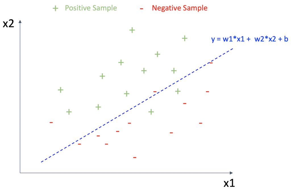
Fig.1 : Linear coefficients for a linear model

The advantages of linear coefficients are 1) it is simple and easy to understand, 2) it explains the “exact” contribution of each feature, and 3) the coefficients are available as model parameters so no additional computation is required. On the other hand, the largest disadvantage of this method is that it is principally applicable to linear models.

Local Linear Approximation

Fig.2 is the same example with Fig.1 but illustrates a non-linear model, y=f(x1,x2) where f is a “black-box” function. One of common techniques to explain such a black-box model is to locally approximate the prediction function by a linear model. For example, the prediction boundary can be approximated by the pink linear model around P1 while it can be approximated by the orange model around P2. 

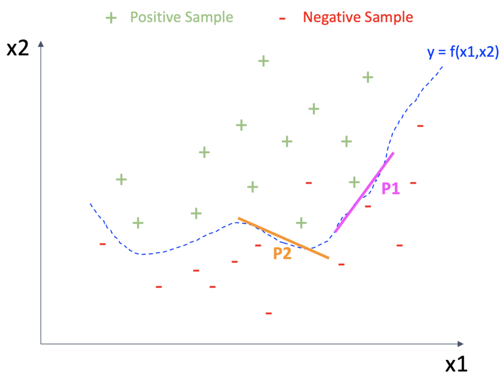
Fig.2 : A nonlinear model and its local explanations

For each “local linear” model, we can apply the “Linear Coefficient” explanation. There are different techniques and LIME may be one of the most common ones. An advantage of this approach is that we can explain any black-box model in principle. However, one of the largest criticisms of this approach is that the linear approximation becomes extremely unreliable when the feature dimensionality is high. It is well known that there are an infinite number of prediction boundaries which achieve the same accuracy when the feature dimensionality is high. In fact, if you add small perturbation to your training data, LIME often returns a very different linear coefficient. 

Feature-wise Evaluation and Permutation Importance

To avoid the curse of dimensionality and measure the impact of each feature reliably, a common technique is to evaluate each feature one by one while still taking into account the other features. The most popular technique might be Permutation Importance which is available in major libraries such as scikit-learn and eli5.

Fig.3 illustrates an idea of permutation importance. To calculate the permutation importance of each feature, we first create another data on which we randomly permute the feature and evaluate the accuracy on this “permuted” data (Accuracy-2 in Fig.3). Because the target feature is randomly shuffled, Accuracy-2 is often worse than the accuracy on the original data (Accuracy-1 in Fig.3). In order to marginalize the random effect, we repeat random permutation several times and calculate the averaged accuracy on the permuted data (Accuracy-2-ave). The permutation importance is defined as the difference between Accuracy-1 and Accuracy-2-ave. Intuitively speaking, the permutation importance measures decrease (or increase) by eliminating the effect of the target feature (x2 in Fig.3).

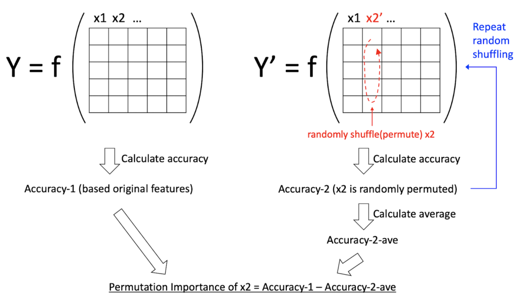
Fig.3 : Permutation importance concept

The permutation importance is generally more robust against feature dimensionality because each feature is evaluated one by one. Also, the procedure is applicable to any black-box models and any accuracy/error metrics. 
While this blog reviewed basic concepts and techniques for AI model transparency, there are more techniques such as SHAP, impurity-based feature importance, or frequency-based feature importance (for gradient boosting). 

Summary
At a fundamental level, model transparency implies explaining the impact of features to final prediction. Some of the common techniques to evaluate features include Linear Coefficients of Features, Local Linear Approximation and Permutation Importance. While linear coefficients are easy to understand and require no computation, they are applicable only to linear models. Using local linear approximation, you can explain any black-box model in theory but linear approximation becomes extremely unreliable when the feature dimensionality is high. The third technique, Permutation Importance seems to be the most popular one as it is available in major libraries. Permutation Importance measures the impact of each feature reliably, evaluating each feature one by one and is robust against feature dimensionality. 
We will discuss Permutation Importance in detail in Part 2 of this blog. Stay Tuned!