
Boost Time-Series Modeling with Effective Temporal Feature Engineering – Part 3
- Technical Posts
Time-series modeling is a statistical technique used to analyze and predict the patterns and behavior of data that change over time. Part 1 of this blog series explained standard time-series models such as AR models, ARIMA, LTSM, and Prophet and discussed their advantages and disadvantages. Part 2, on the other hand, introduced an alternative approach – feature engineering from temporal datasets, that provides numerous benefits over standard time-series modeling.
In Part 3, the last of this blog series, we will examine ARIMA and Prophet models, compare them with an alternative feature engineering approach, and demonstrate the advantages of the feature engineering approaches.
In this blog, we utilized the dataset taken from the Prophet quick start demo guide. The data is a time series based on the log of daily page views for the Wikipedia page for Peyton Manning. The data is a periodic time series spanning eight years (2008 – 2015) and is ideal for demonstrating common time series modeling technologies. Below we see a quick view of the data over time:
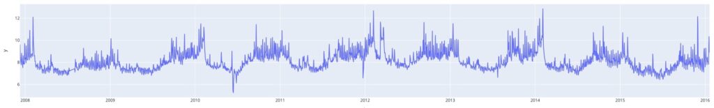
Fig.1 Daily page views for the Payton Manning Wikipedia page
There are some interesting behaviors in the data set:
We forecast the future period of Jan 2015 to Jan 2016 based on the historical data from Dec 2007-Dec 2014. We loaded the dataset as a Pandas Dataframe and sliced it into training and test sets.
import pandas as pd
df = pd.read_csv('https://raw.githubusercontent.com/facebook/prophet/main/examples/example_wp_log_peyton_manning.csv')


# Prepare the data for ARIMA
train = df[df['ds'] < '2015-01-01'] # 7 years of data for training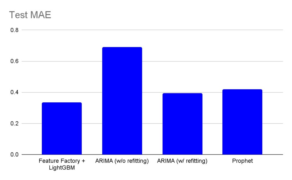
test = df[df['ds'] >= '2015-01-01'] # ~1 year and 1 month of data for testTable.1 summarizes the test MAE scores of four methods that this blog compared.
As shown in the chart, “Feature Factory + LightGBM ” reduced the forecasting error (test MAE) by 15%-20% compared to ARIMA and Prophet. The significant difference in forecasting error demonstrates how powerful the temporal feature approach is in building accurate forecasting models.
Now let’s dive into the details:
Accuracy comparison among three techniques.
As discussed in Part 1, ARIMA and Prophet are very popular time-series models. ARIMA revolves around the idea of modeling time series data by combining autoregressive (AR), differencing (I), and moving average (MA) components as follows:
The above components form the features are then fitted into a linear regression model.
Prophet uses an additive model, which decomposes the time series into three main components: trend, seasonality, and holidays. The model assumes that these components combine linearly to generate the observed values. Compared to ARIMA, Prophet automatically supports more types of features and supports linear and exponential modeling for these features. Features that Prophet automatically detects include:
For ARIMA, we used auto-ARIMA, the auto-ML version of ARIMA that automatically detects the ARIMA components (lags, differencing and moving averages) and then built the ARIMA model. The code snippets of both ARIMA and Prophet can be seen below.
import pmdarima as pm # to detect ARIMA parameters using auto-arima
from statsmodels.tsa.arima.model import ARIMA # to build the ARIMA model


# Auto-ARIMA to detect ARIMA model parameters
model = pm.auto_arima(train.y,
                      start_p=1, start_q=1,max_p=10, max_q=10,
                      m=1, # frequency of series set to annual
                      d=1, # 'd' determined manually using the adf test
                      seasonal=True,
                      start_P=1, start_Q=1, D=0,
                      trace=True,
                      error_action='ignore',
                      suppress_warnings=True,
                      stepwise=True)


# Extracting the ARIMA parameters
model.get_params() #order (7,1,9) is obtained from `get_params()` method


# Build the ARIMA model
model_fit = ARIMA(train.y, order=(7, 1, 9))  # order for AR, I, MA components were obtained from auto-ARIMA
fitted = model_fit.fit()


# Forecast for the test period of 2015 (383 data points)
fc = fitted.forecast(383)
Fig.2 illustrates the actual page views and the predicted page views using ARIMA for the future period of 1 year (Jan 2015 to Jan 2016). We can see that the forecasts (red line) look very different from the actual (blue line). This discrepancy is due to the simplistic nature of the ARIMA model. Namely, ARIMA can capture only one seasonality at a time and completely failed to learn the fluctuations in this data. Another noticeable point is the forecast flatlining after a few months. The reason for this is that in the forecast period, ARIMA uses previous forecasts to calculate future forecasts. Using previous forecasts means ARIMA could be good with short-term forecasts but struggles with long-term forecasts with datasets like the one below.
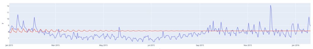
Fig.2 Prediction results of ARIMA without refitting (Jan 2015 to Jan 2016)
A typical workaround is refitting the ARIMA models regularly, depending on the accuracy requirements of the business. Given that we observe weekly seasonality, we could refit the model weekly. Fig.3 illustrates the forecasts of ARIMA with weekly refitting, and we see significant improvement. One of the important drawbacks of this approach is the overhead of rebuilding the model frequently (in this example, weekly).
# Date formatting to allow for weekly refit
date_format_tables = [df, train, test]
for table in date_format_tables:
    table['ds'] = pd.to_datetime(table['ds'])


# Ensuring that we train on a weekly basis by identifying the test time point that is 7 days ahead of train
test['ds_pet'] = test['ds'] - pd.Timedelta(days=7)


#initializing a dataframe to collect the predictions
df_preds = pd.DataFrame(columns = ['ds', 'actual_y', 'test_pred'])


# Rebuilding the model on a weekly basis
for pet, start_date, i in zip(test['ds_pet'], test['ds'], range(len(test))):
  train_rolling = df[df['ds'] < pet]
  test_rolling = df[df['ds'] == start_date]
  model_refit = ARIMA(train_rolling.y, order=(7, 1, 9))
  fitted = model_refit.fit()
  fc_test = pd.DataFrame({'yhat' : fitted.forecast(1)})
  df_preds = df_preds.append({'ds' : start_date,
                   'actual_y' : test_rolling.iloc[0]['y'],
                   'test_pred' : fc_test.iloc[0]['yhat']},
        ignore_index = True)
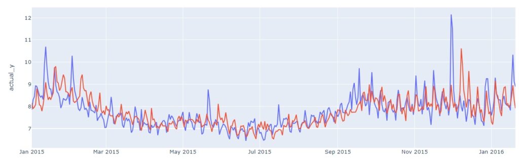
Fig.3 Prediction results of ARIMA with weekly refitting (Jan 2015 to Jan 2016)
Next, we applied Prophet based on the same setting as ARIMA without refitting. Because Prophet can capture multiple seasonal patterns in this dataset, Prophet performed reasonably well without weekly refitting, as illustrated in Fig.4. On the other hand, Prophet’s forecasts are consistently over-predicted. Prophet also assumes that every week has a similar pattern and forces that pattern over time, which may not be the case in a real-world application.
from prophet import Prophet # to build the Prophet model


# Set date column to the right format
train['ds'] = pd.to_datetime(train['ds'])
test['ds'] = pd.to_datetime(test['ds'])


# Build Prophet model
m = Prophet()
m.fit(train)


# Forecast for the test period of 2015 (383 data points)
forecast_for_train = m.predict(train)
forecast_for_test = m.predict(test)
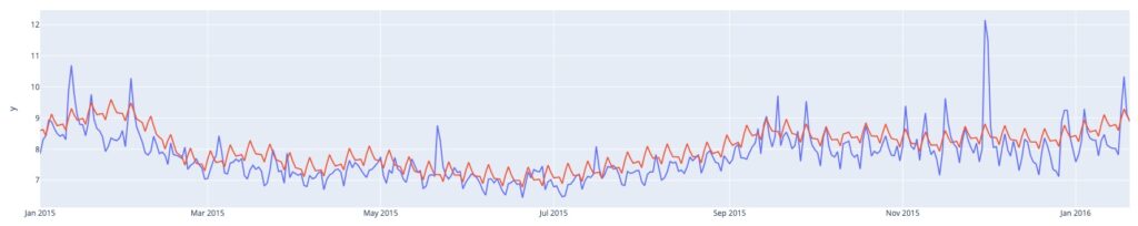
Fig.4 Prediction results of Prophet (Jan 2015 to Jan 2016)
As discussed in Part 2, an alternative approach to time-series modeling is feature engineering. First, feature engineering techniques transform temporal data into a flat feature table. Standard machine learning algorithms train a model based on the feature table.
While conventional feature engineering relies heavily on manual efforts and the intuition of data scientists, dotData provides a data-centric and programmatic feature discovery platform, Feature Factory, designed to extract various time-series features from temporal datasets. We apply dotData’s Feature Factory on this daily view prediction problem and use a LightGBM model on these features.
Feature Factory automatically discovers features over varying time ranges based on the available data, making it easy to account for long-term and short-term forecasting. A sample of the features automatically discovered by Feature Factory for this dataset is shown below:
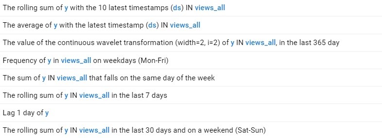
Fig.5 Temporal features detected by dotData Feature Factory
Notice various time ranges and aggregation functions are automatically detected and created for use in the model. Automatic detection and aggregation provide feature engineering transparency and increase business trust.
Based on these temporal features, as Fig.6 illustrates, an alternative approach (dotData Feature Factory + LightGBM) produced the most accurate prediction (for accuracy comparison, see Table 1 in the first part of this blog). dotData detected seasonal and non-seasonal patterns and automatically captured spikes in the time series without manually testing various time points for fluctuations. If we compare this to the Prophet model, we see that the consistent overfit issue observed in Prophet disappears, contributing to the reduction in the MAE test.
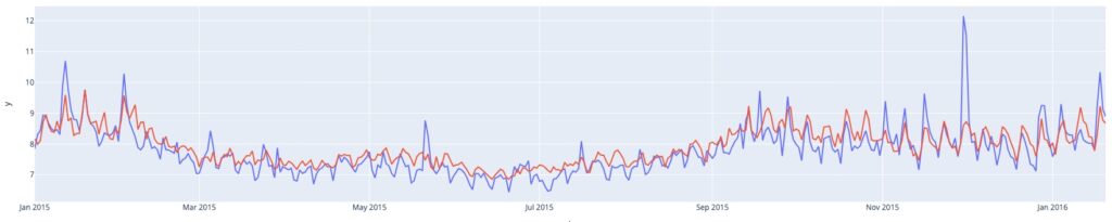
Fig.6 Temporal features detected by dotData Feature Factory
ARIMA and Prophet are great methods for beginners for one-stop time series forecasting but have multiple practical difficulties. Their fundamental challenges lie in the type of time-series features explored, and modeling techniques employed are hard coded in these methods and cannot be customized by users. Lack of customization significantly limits users’ ability to model complex relational time series data and utilize state-of-the-art machine learning algorithms.
An alternative method of feature engineering and state-of-the-art machine learning algorithms can overcome many of the challenges posed by traditional time series models.
Utilizing a data-centric and programmatic feature discovery process to identify features and applying machine learning on them for advanced users to develop forecasting models that are more powerful and incorporate domain knowledge is a paradigm shift.
dotData’s Feature Factory is exceptional at capturing time-series features from complex relational datasets. Feature Factory users can automatically develop predictive time-series features, customize them by incorporating domain knowledge, and apply them to advanced machine learning models, resulting in robust forecasting. If you want to experience the power of Feature Factory, sign up for dotData’s free trial.