
Feature Engineering for Temporal Data – Part 2: Types of Temporal Data
- Technical Posts
Temporal data is one of the most common and essential data types for enterprise AI applications, such as demand forecasting, sales forecasting, price prediction, etc. Analyzing time-series data helps organizations understand underlying patterns in their business over time and allows them to forecast what will happen in the future (a.k.a. time-series forecasting).
Part one of this series focused on standard time-series models such as AR models, ARIMA, LTSM, and Prophet. While time-series modeling techniques are still widely used, they have limitations, such as the inability to work with heterogeneous data characteristics or time resolutions, lack of support for temporal transactions, and poor model explainability and transparency.
This second part will review an alternative approach, i.e., feature engineering from temporal datasets, that provides many advantages over standard time-series modeling. We will look at three different types of temporal data, the alternative approach of engineering new features from the temporal datasets, an overview of some of these features, and how feature engineering eliminates the previously mentioned limitations of the standard method.
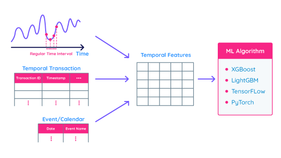
Temporal data is data where a timestamp characterizes each record. Time-series data consist of values with regular time intervals, such as daily stock price, weekly sales, monthly inventory level, etc. Transaction data (or temporal transaction data) is another popular type of temporal data that consists of records of specific transactions with arbitrary time stamps, such as point-of-sales transactions, weblogs, failure alert transactions, etc. Event/calendar data is temporal information containing a collection of events with fixed timestamps, such as payroll dates, holidays, campaign schedules, etc. Figure 1 below summarizes these three types of temporal information.
While the time-series modeling techniques explained in Part I of this series focus almost exclusively on time-series data, the other types of temporal data are critical sources of information.
An alternative approach to time-series modeling is feature engineering. First, feature engineering techniques transform temporal data into a flat feature table. Standard machine learning algorithms train a model based on the feature table. While time-series modeling techniques capture time-series behaviors inside their models, this alternative approach encodes temporal information into features.
This simple feature engineering approach overcomes various drawbacks of time-series modeling techniques and offers greater flexibility to develop better time-series/temporal prediction models. For example, we can apply aggregation functions with different time resolutions to handle data with heterogenous time resolutions and other encoding techniques to time series with different data characteristics (e.g., simple mean encoding for numeric time series vs. categorical count encoding for categorical sequence). The feature engineering approach provides a natural way to integrate transaction and event/calendar information into a single feature table. Feature engineering also allows for control of the balance between the complexity of features and the accuracy of the final models and leverages existing techniques in machine learning to secure the transparency and interpretability of your models.
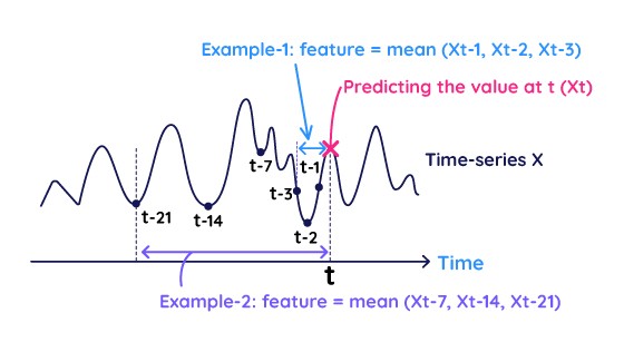
Temporal aggregations are basic yet very flexible ways to derive features from time series and transaction data. Two consideration points define temporal aggregation features: 1) what ranges and lags of data to aggregate, and 2) how to aggregate multiple records in the selected range.
Figure 2 illustrates examples of temporal aggregation features. Example 1 generates features by aggregating the latest records (almost equivalent to the auto-regressive modeling explained in Part I). Example 2 generates features by aggregating the periodic records in 7-day cycles to capture weekly patterns. This (e.g., weekly patterns, seasonality, etc.). While these examples use “mean” as their aggregation functions, different aggregations (max, min, stdev, etc.) can extract other temporal behaviors (and thus different features).
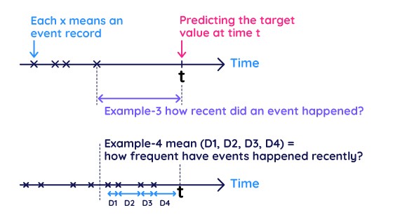
Time IntervalTime intervals are also powerful ways to derive features from transaction data. Figure 3 illustrates two examples of time interval features. Example-3 measures how recently events happened (time interval to the latest record), while Example-4 measures how frequently certain events happened (averaged time interval during a fixed time period). These time interval features are highly related to RFM (recency, frequency, and monetary) models in consumer marketing and behavior analysis. Time interval features can be extracted based on two specific timestamps. For example, in the NY City Taxi dataset (a very famous Kaggle competition), the interval between “pick-up time” and “drop-off time” express the travel time that is highly correlated with the fare.
A timestamp itself can become a good feature. For example, we can convert “3/15/2022 09:00:00” into categorical values such as “March” or “Morning” and then apply categorical-value encoding techniques. Such timestamp featurization extracts contextual information from raw timestamps and ocastionally helps improve model performance. Another common approach is to create binary flag features from event/calendar information. For example, we can convert a timestamp into a holiday flag feature based on the holiday calendar. It is well-known that such a holiday flag feature significantly improves the accuracy of holiday product demand (e.g., retail product sales on Black Friday).
There are more ways to extract temporal features. Exponentially Weighted Moving Average (EWMA) is widely used in time-series volatility analysis and captures longer-term moving average effects. Fourier transformation is commonly used in manufacturing sensor data and captures time-series characteristics in a frequency domain. Continuous wavelet transform extracts features in both frequency and time domains. The number and variety of available temporal features continue to grow, and the feature engineering approach can leverage them (OSS such as tsfresh provides various temporal features as a library.)
In modern time-series modeling, the feature engineering approach has become more popular than traditional time-series modeling. The advantage of the feature engineering approach to time-series problems is the flexibility of designing arbitrary features and incorporating more information to your model. In Part III, we will discuss some challenges of the feature engineering approaches and how to address them.
Learn more about how your organization could benefit from the powerful features of dotData by signing up for a demo.