Fast and More Robust Permutation Importance for Black-box Model Transparency on Imbalanced and High-Dimensional Data

In the first part of this blog, Basic Concepts and Techniques of AI Model Transparency, we reviewed a few common techniques for AI model transparency such as linear coefficients, local linear approximation, and permutation importance. In particular, the permutation importance is applicable to any black-box models, any accuracy/error functions, and more robust against high-dimensional data (because it handles each feature one by one rather than all features at the same time).

One of the drawbacks of the permutation importance is its high computation cost. We have to repeat the evaluation process by (the number of features) * (the number of random shuffling to repeat) * (the number of models). To reduce the computation time, a common approach is to apply downsampling that works well when the positive and negative classes are balanced. However, such naive downsampling makes permutation importance extremely unreliable. 

Permutation Importance Under Class Imbalance

Let us first see how unstable the permutation importance becomes using a naive downsampling based on the Kaggle’s Credit Card Fraud Detection dataset. The dataset, that has been upvoted on the platform almost 6000 times, is a famous example of a classification use case with imbalance classes. The objective was to detect fraudulent transactions building a model on data that contained only 492 frauds out of 284,807 transactions that occurred in two days (0.17% positive samples). There are 30 features, namly V1, V2, …, V28, Time and Amount. The experimental settings are summarized as follows: 

• The experiments below were performed on a standard laptop computer with Intel Core i7-9750H CPU (6 cores);
• We used eli5 and XGBoost; 
• We used AUC as the accuracy metric (Area Under the Curve of Receiver Operating Characteristic); 
• The number of shuffles was set to 5 (the default value of eli5).

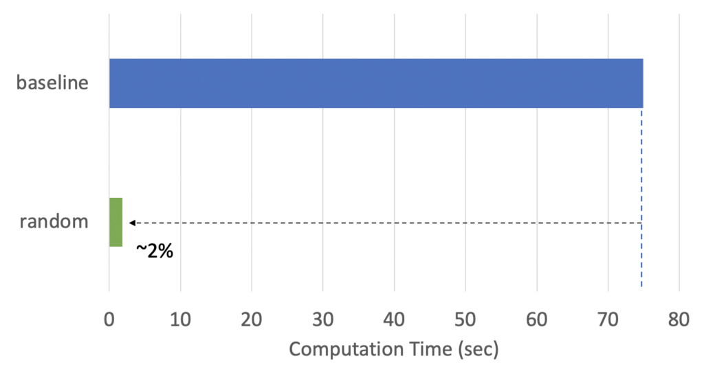
First, Fig.4 shows the computation time of the permutation importance. The “baseline” used eli5 without downsampling. As we see, it took about 75 seconds to compute permutation importance. Although you may feel 75 seconds is acceptable, imagine the dataset contains 300 features rather than 30 and you have 10 models on which you want to compare permutation importance. Then, the computation time to calculate the permutation importance becomes 7,500 seconds which is more than 2 hours. A reasonable way to reduce computational time is to apply downsampling. The “random” applied random sampling which randomly extracted 5,000 samples (~1.7% of the original population). As can be seen in Fig.4, the computation time decreased proportionally. 
 

Fig.4 : Computation time of permutation importance on the Credit Fraud Detection dataset. The “baseline” method just used eli5 without downsampling while the “random” method applied 1.7% down sampling (5,000 samples).

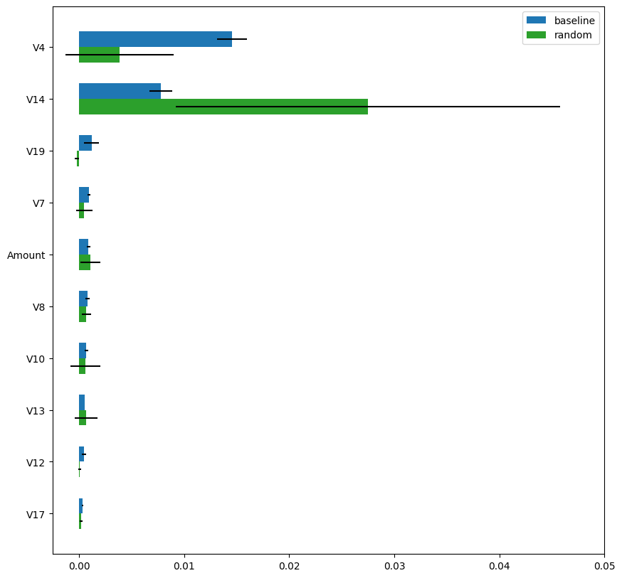
Next, Fig.5 shows the estimated permutation importance for “baseline” (blue) and “random” (green). As shown, the permutation importance values of the “random” method are very different from those of the “baseline” method. Moreover, the estimation variance (standard deviation across 5 random shuffles) is extremely large and the permutation importance estimated using the “random” method is unreliable.

Fast and Stable Permutation Importance

The main reason for this instability is the lack of positive samples after downsampling. In the Kaggle’s Credit Card Fraud Detection dataset, only 8-9 positive samples (1.7% of 492 positive samples) are included on average after downsampling. Thus, every random shuffle is evaluated based on only 8-9 positive samples and you can imagine how unstable the permutation importance becomes. You may consider to apply balanced (or stratified) sampling to have more positive samples. However, such balanced (or stratified) sampling changes the class distribution. In other words, the positive and negative sample ratio changes before and after the sampling and eventually makes accuracy calculation inappropriate.
At dotData, we implement our own fast and stable algorithm to compute permutation importance under class imbalance. Although this blog does not dive into technical details of the algorithm, the idea is summarized as follow: 

• Apply stratified sampling to extract more positive samples while reducing the size of the entire population. 
• Apply theoretical adjustment of the distribution change induced by the stratified sampling to calculate accuracy.

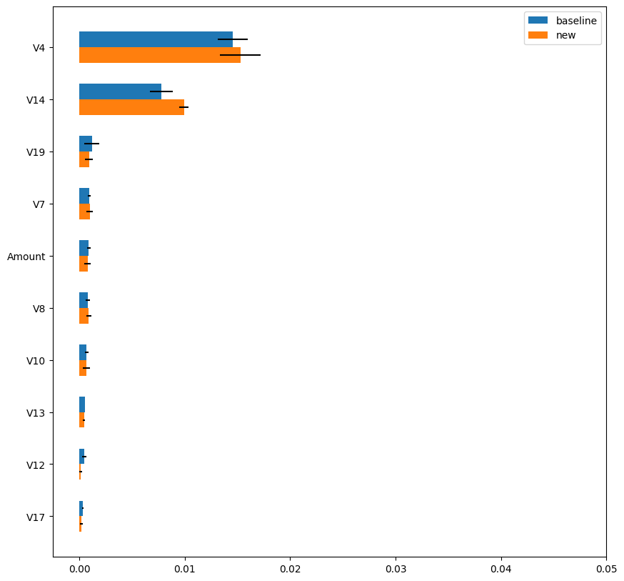
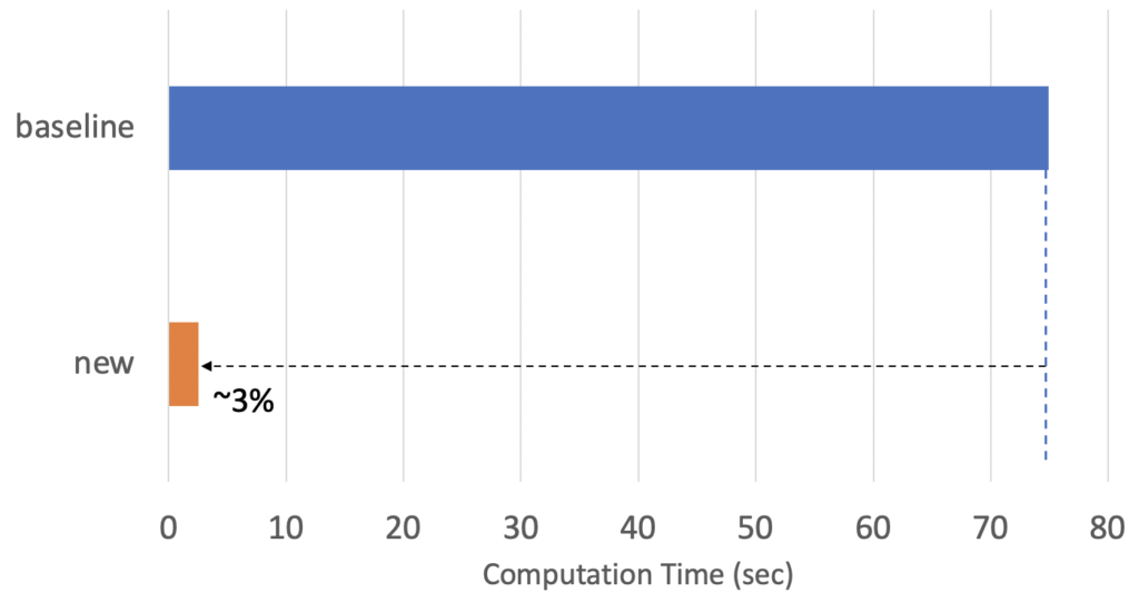
Fig.6 compares the permutation importance values calculated using the “baseline” method and the “new” method. As can be seen, the “new” method returned very similar estimation results as the “baseline” method and the estimation variance is much smaller than that of the “random” method (see Fig.5). Fig.7 shows the computation time of the “new” method. The computation time of the “new” method is only 3% of the “baseline” method and achieved more than 30x speed-up with stable and reliable estimation.

Fig.6 : Top-10 permutation importance values estimated
using the “baseline” and “new” methods.

Key Takeaways

In this two-part blog series, we have discussed how to improve transparency of black-box models on unbalanced data. The key takeaways are: 

• Model transparency is one of the most fundamental and important aspects of any AI/ML models in enterprise due to various reasons such as explainability for model consumers, accountability in regulated industries, and so on (see our white paper for more discussions.)
• For many practical classification applications, class labels are highly unbalanced. On such imbalanced data, many common model transparency methods become highly unreliable (or computationally too demanding to be practical).
• dotData developed a proprietary algorithm that significantly improves both stability and computation time to provide better model transparency on imbalanced and high-dimensional data (the algorithm was implemented in dotData Enterprise 1.6 / dotData Py 1.2 or later.)